用 Python 建模热力学熵
熵是热力学系统的一种属性,在可逆绝热过程中保持不变。此外,我们还可以说它是系统中随机性或无序性的程度。如果系统在温度 T 下从周围环境交换 dQ 热量,则熵的机会可以写为 −
$$\mathrm{ds \: = \: \frac{dQ}{T} \dotso \dotso \: (1)}$$
根据克劳修斯不等式,沿可逆路径的 $\mathrm{\frac{dQ}{T}}$ 的循环积分小于或等于零。从数学上来说,它可以写成 −
$$\mathrm{\oint\frac{dQ}{T} \: \leq \: 0\dotso \dotso \: (2)}$$
等式适用于可逆循环,不等式适用于不可逆循环。任何不遵循等式 2 的发动机循环都是不可能的。
对于不同类型的过程,熵变化的评估方式不同。在显热相互作用过程中,由于没有相变,只有温度变化,因此从状态 1 到状态 2 的变化熵可以写成 −
$$\mathrm{\triangle S \: = \: mc_{p} \: In \: (\frac{T_{2}}{T_{1}})\dotso \dotso \: (3)}$$
其中,$\mathrm{c_{p}}$ 是恒压下的比热容。而如果存在相变,则温度不会改变,因此熵可以简单地计算为潜热除以相变温度,如下所示 -
$$\mathrm{\triangle S \: = \: \frac{mL}{T}\dotso \dotso \: (4)}$$
其中,L 是比潜热。等式中提到的熵。 3 和 4 是总熵,即单位为 kJ/K,但在大多数情况下,我们处理的是特定属性,因此特定熵 (kJ/kg-K) 用小 s 表示,定义为 −
$$\mathrm{s \: = \: \frac{ds}{dm}\dotso \dotso \: (5)}$$
在一个过程中,如果气体的状态从压力和温度 $\mathrm{p_{1} \: , \: T_{1}}$ 变为 $\mathrm{p_{2} \: , \: T_{2}}$,则特定熵的变化可以写为 −
$$\mathrm{\triangle s \: = \: c_{p} \: In \: (\frac{T_{2}}{T_{1}}) \: − \: R \: In \: (\frac{p_{2}}{p_{1}})\dotso \dotso \: (6)}$$
在很多情况下,使用熵可以非常轻松地解决问题。这些特殊情况是 −
当两个温度分别为 $\mathrm{T_{1}}$ 和 $\mathrm{T_{2}}$ 的相同系统通过可逆引擎连接时,从这些有限体获得的最大功及其最终平衡温度将由 −
$$\mathrm{W_{max} \: = \: C \: \times \:(\sqrt{T_{1}} \: − \: \sqrt{T_{2}})^{2}\dotso \dotso \: (7)}$$
$$\mathrm{T_{eq} \: = \: \sqrt{T_{1} \: \times \: T_{2}}\dotso \dotso \: (8)}$$
其中,C 是系统的热容量,是质量和比热的乘积。
在混合两种具有相同热容量 (C) 和不同温度 $\mathrm{T_{1} \: 和 \: T_{2}}$ 的流体时,整个系统的熵变将由 −
$$\mathrm{\triangle S \: = \: C \: In \:(\frac{(T_{1} \: + \: T_{2})/2}{\sqrt{T_{1}T_{2}}})\dotso \dotso \: (9)}$$
通过可逆发动机连通的系统(温度为 T)和热能储存器(温度为 $\mathrm{T_{0}}$)可获得的最大功为 −
$$\mathrm{W_{max} \: = \: C \:((T_ \: − \: T_{0}) \: − \: T_{0} \: In \: (\frac{T}{T_{0}})\dotso \dotso \: (10)}$$
用于模拟热力学熵的 Python 程序
以下函数用 Python 编写,用于执行不同情况下的熵计算 −
相变过程中的熵变化
def s_pc(T,L):
    return L/T
显热能传递过程中的熵变化
def s_se(c,T1,T2,m=1):
    return m*c*log(T2/T1)
模拟克劳修斯不等式
def clausius_inequality(Q,T):
   Sm=sum(Q/T)
   if Sm<0:
      print("The cycle is irreversible and possible")
   elif Sm==0:
      print("The cycle is reversible and possible")
   else:
      print("The cycle is not possible")
有限热容量物体可获得的最大功
def max_work_fb(T1,T2,c):
    Tf=sqrt(T1*T2)
    work=c*(sqrt(T1)-sqrt(T2))**2
    return work,Tf
有限热容量物体与热能库相互作用可获得的最大功
def max_work_fb_TER(T,T0,c):
    return c*((T-T0)-T0*log(T/T0))
给定压力和温度变化过程中气体的熵变化。
def s_process(T1,T2,p1,p2,R,cp):
    return cp*log(T2/T1)-R*log(p2/p1)
绘制相变过程(液体到蒸汽)的 T-S 图的函数
def plot_pc(Δs1,Δs2,Δs3,Ti,Tpc,Tf):
   # Plotting cycle
   s1=0
   s2=s1+Δs1
   s3=s2+Δs2
   s4=s3+Δs3

   # 1-2
   s=linspace(s1,s2,10)
   T=empty(len(s))
   T[0]=Ti

   for i in range(1,len(s)):
      T[i]=T[i-1]/(1-(s[1]-s[0])/ci)
   plot(s,T,'r-')

   # 2-3
   s=linspace(s2,s3,20)
   T=zeros(20)+Tpc
   plot(s,T,'b-')

   # 3-1
   s=linspace(s3,s4,20)
   T=empty(len(s))
   T[0]=Tpc

   for i in range(1,len(s)):
      T[i]=T[i-1]/(1-(s[1]-s[0])/cw)
   plot(s,T,'g-')
   xlabel('S')
   ylabel('T')
   savefig("Entropy_pc_jpg")
   show()
除了这些之外,还有一个非常有用的功能,那就是过程中的热量相互作用量(涉及显热和潜热)
#-----------------------------------------------
# 相变过程中的热传递
#-----------------------------------------------
def q_mel_sol(m,Ti,Tf,T_pc,c_bpc,c_apc,L):
   """
   Function for the evaluation of heat transfer during phase change
   Input : mass (m), initial temp (Ti), final temp (Tf),
   phase change temp (T_pc),sp. heat below phase change (c_bpc),
   sp. heat above phase change (c_apc), latent heat (L)
   Output: heat interaction
   """
   if Ti>Tf:
      print('Process is either freezing or condensation')
      return m*(c_bpc*(T_pc-Ti)-L+c_apc*(Tf-T_pc))
   else:
      print('Process is either melting or vaporization')
      return m*(c_bpc*(T_pc-Ti)+L+c_apc*(Tf-T_pc))
现在让我们举几个问题来演示上述函数的使用。
示例 1
一个引擎在 400 K 时接收 105 kJ,并在 200 K 时拒绝 42 kJ。检查引擎是否可行。
解决方案
我们将使用函数 clausius_inequality() 来检查该过程的有效性。
程序和程序的输出如下 −
代码 |
输出 |
|---|---|
from numpy import * Q=array([105,-42]) T=array([400,200]) clausius_inequality(Q,T) |
循环不可能 |
示例 2
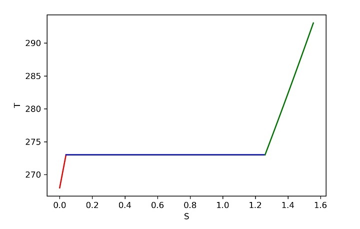
1 千克 268 K 的冰通过从 298 K 的大气中吸收热量转化为 293 K 的水。冰和水的比热分别为 2.093 和 4.187 kJ/kg-K。如果冰的熔点为 273 K,则计算冰、周围环境和宇宙的熵变。此外,在 T-s 图中绘制该过程。(相变期间的潜热为 333.3 kJ/kgK)
解决方案
from pylab import *
# 初始冰温。
T1=268

# 相变温度。
T2=273

# 最终水温。
T3=T0=293

# 冰的比热
ci=2.093

# 水的比热
cw=4.187

# 融化过程中的潜热
L=333.3

# 1-2 冰
Δs1=s_se(ci,T1,T2,m=1)

# 2-3 相变
Δs2=s_pc(T2,L)

# 3-4 水
Δs3=s_se(cw,T2,T3,m=1)

# 系统熵变
Δs_ice=Δs1+Δs2+Δs3

# 来自大气的热传递
Q=q_mel_sol(1,T1,T3,T2,ci,cw,L)

# 周围环境熵变
Δs_atm=-Q/T0

# 系统熵变宇宙
Δs_uni=Δs_ice+Δs_atm
print("Δs_system = ",round(Δs_ice,4))
print("Δs_surr = ",round(Δs_atm,4))
print("Δs_uni = ",round(Δs_uni,4))

# 绘制 T-S 图
plot_pc(Δs1,Δs2,Δs3,T1,T2,T3)
输出
程序输出将是 −
过程是熔化或汽化
Δs_system = 1.5556
Δs_surr = -1.4591
Δs_uni = 0.0965
它还将生成以下图 −
结论
在本教程中,使用 Python 编程对热力学熵进行了建模,并且已在数值问题上实现和测试了开发的函数。